Graphing

Graphing in VPython is dynamic and can be done in real time. For example, points can be added to a plot of x vs. t as an object moves. Histogram bars can be adjusted as distributions change.

Terminology

A graph is a 2D canvas on which plots of various kinds can be displayed.

A gcurve object is a continuous curve connecting data points.

A gdots object displays data as discrete points.

A gvbars object displays discrete vertical bars, and a ghbars object displays discrete horizontal bars.

graph

A graph is a 2D region in which 2D data can be plotted, analogous to a 3D canvas in which 3D objects are displayed. As in the case of canvas, the actual data display objects belong to a specific graph. Multiple graphs can be created.

If you create a data object such as a gcurve without first creating a graph, VPython will automatically create a graph for you. This is convenient for simple, rapid graphing. The advantage to creating a graph explicitly is that it can be given a title, caption, or key, and its alignment can be specified.

g1 = graph(title='My Graph', xtitle='x', ytitle='t', xmin=0, ymin=-20 )

Parameters:

• title (string) – Title of the graph. html formatting for sub, sup, italic allowed.

• xtitle (string) – Title of horizontal axis. html formatting for sub, sup, italic, bold allowed. (e.g. ‘<i>t</i>’).

• ytitle (string) – Title of vertical axis. html formatting for sub, sup, italic, bold allowed. (e.g. ‘x₁’).

• xmin (scalar) – Minimum value on horizontal axis. Default: graph will adjust automatically as points are added.

• xmax (scalar) – Maximum value on horizontal axis. Default: graph will adjust automatically as points are added.

• ymin (scalar) – Minimum value on vertical axis. Default: graph will adjust automatically as points are added.

• ymax (scalar) – Maximum value on vertical axis. Default: graph will adjust automatically as points are added.

• width (scalar) – Width of graph in pixels. Default 640.

• height (scalar) – Height of graph in pixels. Default 480.

• background (vector) – Color of background. Default color.white.

• foreground (vector) – Color of foreground (axes, labels, etc.). Default color.black.

• align (string) – Placement in window. Options ‘left’, ‘right’, ‘none’. Default is ‘none’.

• scroll (boolean) – If True, points are deleted from one end of the plots in the graph as they are added to the other end (a chart recorder). You must specify the initial xmin and xmax, where xmax > xmin.

• fast (boolean) – If True, plotting is faster but fewer graph inspection options are available. Default True. See Plotting Packages.

• logx (boolean) – If True, plots on a log scale. All values must be positive. Only available with fast=False.

• logy (boolean) – Same as logx, for vertical axis.

graph methods

mygraph.select()

Makes this the current graph.

mygraph.delete()

Deletes this graph and all its contents.

current = graph.get_selected()

Returns the currently selected graph (the one to which new gcurves etc. will belong)

gcurve

A gcurve displays a list of data points as a continuous curve.

gc = gcurve(color=color.red)

Parameters:

• color (vector) – Color of this gcurve. Default is color.black.

• label (string) – Text identifying this gcurve. Appears at upper right in color of this gcurve.

• legend (boolean) – If True, labels are displayed. Default True.

• width (scalar) – Width of line in pixels.

• markers (boolean) – If True, dots displayed at each data point.

• width – Width of dot used for markers. Default slightly larger than gcurve width.

• marker_color (vector) – Color of marker dots. Default is the gcurve color.

• dot (boolean) – If True, the most recent point plotted is highlighted with a dot. Useful if a graph retraces its path.

• dot_radius (scalar) – Width of dot in pixels. Default is 3.

• dot_color (vector) – Color of dot. Default same as gcurve.

• visible (boolean) – If True this object is displayed. Default True.

• data (list) – A list of (x,y) pairs to populate the gcurve. If used after creation, gc.data=[ … ] will replace any existing data in the gcurve.

• graph (object) – The graph to which this object belongs. Default: most recently created graph.

gcurve methods

Plotting a data point:

gc.plot(x, y)

Parameters:

• firstargument (scalar) – Value on horizontal axis.

• secondargument (scalar) – Value on vertical axis.

The point (x,y) is added to the end of the gcurve.

Alternate form of plot():

gc.plot( [ (1,2), (2,3), (3,4) ] ).

Data pairs can be tuples or lists.

Deleting a gcurve:

gc.delete()

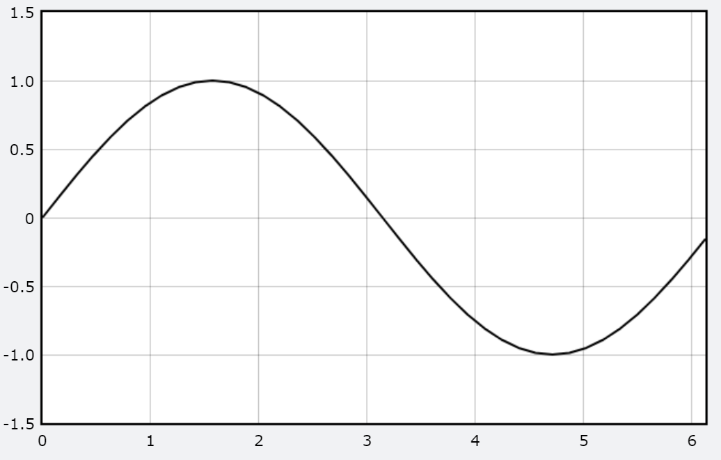
A Simple Plot

The following VPython program plots a sin function. Note that no graph is explicitly created.

a = gcurve()

for x in arange(0, 2*pi, pi/20):
        rate(30)
        a.plot(x, sin(x))

Several gcurves (or gdots or gvbars) can be plotted on the same graph.

gdots

A gdots object will display a list of (x,y) pairs as discrete points instead of as a connected curve.

gd = gdots(color=color.red)

Parameters:

• color (vector) – Color of this gcurve. Default is color.black.

• radius (scalar) – Radius of a dot in pixels. Default 3.

• size (scalar) – The diameter of a dot in pixels.

• label (string) – Text identifying this gdots. Appears at upper right in color of this gcurve.

• legend (boolean) – If True, labels are displayed. Default True.

• visible (boolean) – If True this object is displayed. Default True.

• data (list) – A list of (x,y) pairs to populate the gdots. If used after creation, gd.data=[ … ] will replace any existing data in the gdots.

• graph (object) – The graph to which this object belongs. Default: most recently created graph.

Methods for gdots are the same as for gcurve.

gvbars and ghbars

A gvbars object displays a vertical bar for each (x,y) data point. A ghbars object displays horizontal bars. The syntax and options are the same.

gv = gvbars(delta=0.05, color=color.blue)

Parameters:

• delta (scalar) – Width of the bar. Default 1.

• color (vector) – Color of the bars. Default is color.black.

• label (string) – Text identifying this gvbars. Appears at upper right in color of this gcurve.

• legend (boolean) – If True, labels are displayed. Default True.

• visible (boolean) – If True this object is displayed. Default True.

• data (list) – A list of (x,y) pairs to populate the gvbars. If used after creation, gv.data=[ … ] will replace any existing data in the gvbars.

• graph (object) – The graph to which this object belongs. Default: most recently created graph.

Methods for gvbars and ghbars are the same as for gcurve.

Plotting Packages

You can choose between two graphing packages, one which is faster (currently based on Flot), or one which offers rich interactive capabilities such as zooming and panning but is slower (currently based on Plotly). The default is the fast version, corresponding to specifying fast=True in a graph, gcurve, gdots, gvbars, or ghbars statement. To use the slower but more interactive version, say fast=False. In many programs the “slow” version may run nearly as fast as the “fast” version, but if you plot a large number of data points the speed difference can be significant.

Do try fast=False to see the many options provided. As you drag the mouse across the graph with the mouse button up, you are shown the numerical values of the plotted points. You can drag with the mouse button down to select a region of the graph, and the selected region then fills the graph. As you drag just below the graph you can pan left and right, and if you drag along the left edge of the graph you can pan up and down. As you move the mouse you’ll notice that there are many options at the upper right. Hover over each of the options for a brief description. The “home” icon restores the display you saw before zooming or panning. Try this demo.

Histograms

The program HardSphereGas provides an example of a dynamic histogram.